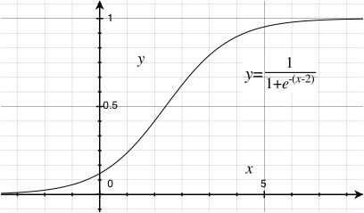
 Figure 1: A `squashed sigmoidal' neuron activation function
Biological neural networks are the webs of neurons that wire the bodies of animals and form their brains. Each neuron is a sophisticated device that acts as a cable, a switch and a memory cell. It receives electrical signals from built-in sensors or from other neurons, processes this input and responds with a signal of its own. The output signal travels down the neuron's long axon, which branches and makes contacts called synapses with other neurons, stimulating (or inhibiting) them in turn. The type of processing a neuron does to its input can generally be adjusted to help the network learn a task or encode a memory. Biological neural networks can contain billions of neurons, trillions of synapses and their computations can be unfathomably complex.
Artificial neural networks are algorithms based on physical models of real neurons and their networks, that hopefully capture some of their computational properties. In the forthcoming example we'll use a crude (but popular) model in which the activity of a neuron is determined by a weighted sum of the activities of the upstream neurons. The weights form the memory; the network `learns' by adjusting these weights (synapses) so to encode a pattern or improve its performance at some task. Our weight-adjusting algorithm will be a variant on the famous Hebbian learning rule, in which activating synapses between two neurons are strengthened if the neurons' activities are correlated, and weakened otherwise. This learning rule, inspired by observations of real neurons, tends to drive the network towards an ordered state, and is thus useful for memorizing patterns.
To summarize, our network will operate in two modes: computation, and learning. In the computing mode, certain input neurons' activities are fixed by the user, while the activities of the other neurons xi evolve by the following formula:
xi = f(∑j Wij xj + bi)
Here xi is, say, the mean frequency of signals of neuron i, Wij is the strength of the synapse from neuron j to neuron i, and bi is called a bias, which is a free parameter can also be trained. The sum runs over all neurons j feeding into neuron i, including the input neurons. The function f is called an `activation function', which we will take to be the same for all neurons. Specifically, we'll use the common activation function f shown in Figure (1). Note the nonlinearity of f: that is what gives the neural network its power.
Figure 1: A `squashed sigmoidal' neuron activation functionIn the training (learning) mode, the neurons' activities stay frozen in time while their weights and biases are updated:
Wij = Wij + η xi xj
bi = bi + η xi
The parameter η determines the learning rate, which must be large enough to train quickly, but not so big that the algorithm overshoots and destabilizes the network.
We will actually use a variant (J. R. Movellan, Contrastive Hebbian learning in interactive networks, 1990) of the basic Hebbian rule which increments the weights by both positive and negative Hebbian steps. The positive step is taken as the network is being `taught'; i.e. the output neurons are held at the values that we would like them to take. The anti-Hebbian update is made after the network does what it wants without the clamping. Heuristically, the network learns what we want it to do and unlearns its old bad habits in separate steps. It can be shown that for the symmetric networks (wij = wji) that we will exclusively work with, this combination of positive and negative reinforcement encodes memories more directly than the basic Hebbian rule would.
The two basic operations of a neural network---propagation of signals to perform computation, and adjustment of the weights---are pretty simple routines, but since they will be repeated many times they can be time-consuming. We should write that part of our program in low-level C code.
Last update: July 28, 2013